Abstract. This article describes a method for object and terrain visualization by means of the combination of two algorithms, one for terrain and one for objects. Our purpose is to generate, efficiently and rapidly, aerial images of terrain with objects such as houses, vehicles, and transmission lines, thus allowing a simulated flight. For the objects, described by lines and polygons, the Z-Buffer algorithm is used; for the terrain, described by height maps, an optimized Ray-Casting algorithm, called Floating Horizon algorithm, is used.
Keywords: Terrain Visualization, GIS, Voxel-Based Modeling, Ray Casting, Interactive Visualization.
In this kind of application, we are primarily concerned with algorithm performance, in order to make interactive navigation possible. An obstacle to be tackled is that the detailed geometry and texture representation of a terrain that is to be flew over demands a large amount of memory. Moreover, even though the portion of the terrain involved in a scene represents, generally, a small part of this information, its visualization using a generic graphical system may not yield the necessary efficiency. Such issues have motivated researches both in techniques for compact vector or raster terrain representations, and in optimized visualization algorithms ( [LaMothe95] and [Freese+95] ).
In the present work we consider the situation in which the scene contains, apart from the terrain, vector objects represented by polygons and lines. These objects can be visualized very efficiently by the standard graphical systems available in modern workstations and PCs, such as OpenGL.
We have compared the results obtained with two approaches for scene visualization containing terrain and vector objects. The first one consists in using the OpenGL graphical system for visualizing both terrain and objects. The second approach consists in using an optimized algorithm for visualizing the terrain; the image and the depth information obtained are then transferred to OpenGL, to be integrated in the scene containing the objects. Comparative results of both approaches are presented.
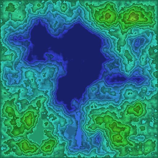
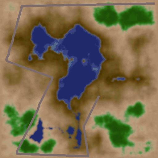
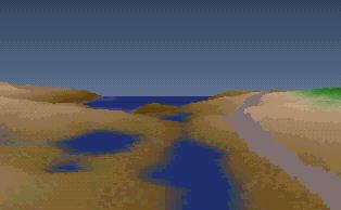
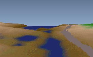
The computer representation of a terrain involves, necessarily, some form of discretization, either by means of a grid (usually regular) or of a Triangular Irregular Net (TIN). In the present work, terrain are represented by regular grids described by two two-dimensional matrices of equal dimensions, one determining the height at each point (height map) and the other determining the texture (color map). Examples of these maps are illustrated in Figure 1. These images were generated by the VistaPro program [VistaPro] and altered to include the highway. The images generated by VistaPro have an implicit illumination, which contributes to increase the degree of realism without degrading the visualization algorithm with expensive illumination models.
The form of representation described above immediately provides a geometric model for a terrain, which can be considered as a set of rectangular blocks aligned by the axes, with width and length equal to the width of each element of the regular grid and height given by the corresponding value on the height map. If we associate to each face of each of these blocks the color provided by the corresponding element on the texture map, we will have a vector model of the terrain, which can thus be visualized by means of a generic system such as OpenGL. The advantage of this approach is the immediate integration of vectorial objects to the terrain, since the same description is used for the terrain and for the objects. The great disadvantage is the large number of faces to be visualized, which can obstruct the interactive visualization. Such issues are discussed in Section 3.
An alternative consists in looking at the terrain through the volumetric perspective. In this case, we consider that the blocks describe space occupation by the terrain. Due to this interpretation, in the games literature ( [Freese+95] and [LaMothe95] ) it is common to call each of these blocks a voxel (volume pixel). As will be seen in Section 4, image-based volume visualization algorithms can be optimized for terrain visualization, fulfilling the interactive visualization requirement. The use of such algorithms, however, is made difficult by the presence of vector objects to be added in scene. One solution is obtaining a volumetric representation of the objects to be put in scene, as is proposed in [tvcg+96]. Such solution, nevertheless, apart from involving considerable pre-processing effort, does not work for arbitrary objects: the terrain structure must be preserved after placing the objects. In other words, each object must lie on the terrain and each vertical straight line with points common to the terrain must intersect it according to a segment having an end on the terrain.
Other suggestions for simultaneous visualization of terrain and objects are presented in [Cohen+94], [Graf+94], [Paglieroni+94] e [GuGaCa97]. [Sawyer97] describes a use for interactive visualization of terrain with objects in games such as flight simulators.
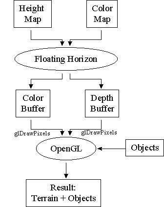
In Section 5 we will investigate another alternative for incorporating vector objects to terrain, in which terrain and objects are processed separately, making use of efficient algorithms for each kind of data. The resulting images of each process are then combined into only one image, taking into account depth information extracted from each algorithm.
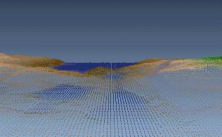
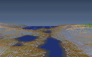
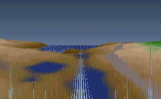
Figure 2 illustrates the images obtained by the Z-Buffer algorithm for each of the above representations. Table 1 shows the time, in seconds, to render each of the images of Figure 2 using a PC PENTIUM 166MHz and a Silicon Indigo 2.
All times shown in Table 1 are too large to support interactive visualization. To reach an interactive time, of 5 frames per second, they must be reduced by a factor greater than 10. Thus, the vector representations of the terrain presented above yield unacceptable performance with the computers largely available today.

| Terrain represented by | PC | SGI |
| [a] Points on top faces | 1.6 | 1.2 |
| [b] Top faces | 3.5 | 2.0 |
| [c] Frontal faces | 4.2 | 2.1 |
| [d] Straight line segments | 2.3 | 2.2 |
| [e] Blocks | 14.2 | 6.2 |
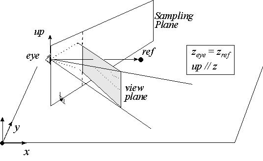
We will assume that the observer's head is vertical and the projection plane is perpendicular to the xy terrain grid, as shown in Figure 3. In this position the rays casted from the observer's eye to each column of pixels in the view plane are contained in a plane which is also perpendicular to the xy plane. This plane, indicated in Figure 3 as sampling plane, largely simplifies the visualization problem. Only the terrain voxels which are intersected by this plane can influence the color of the view plane column's pixels. Furthermore, if the voxels are sampled at uniform spaces along the intersection, the projection is reduced to a simple 2D problem, as illustrated in Figure 4.
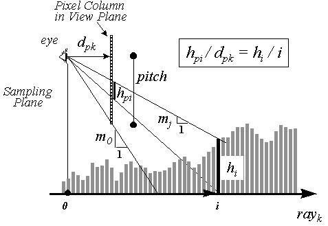
Algorithms that explore the terrain's particular model can be easily found in game programming literature [LaMothe95] and [Freese+95]. These algorithms treat each screen column separately and paint, for each column, the pixels from the bottom of the screen upward, following the idea of a floating horizon. The Floating Horizon Algorithm starts by casting the first horizon, shown as m0 in Figure 4. In order to determine the color of the bottom screen pixel, the algorithm tests the height of each column starting at the observer's foot, marked as O in Figure 4, and moving forward in the rayk direction. The first column which raises above the horizon causes the pixel to be painted and the horizon to move upward. The algorithm uses the fact that terrain voxels which are further away in the rayk direction can not obscure the pixels already painted.
An implementation of the Floating Horizon Algorithm for a pixel column is illustrated in Algorithm 1.
Note that, as we move from one position i to the next, the horizon height decreases by the value of the current horizon slope, mj, as shown in line 6 of Algorithm 1.
Figure 4 also shows that the slope of the first horizon is given by:
m0 = pitch / dpk (1)
and the change in the slope, as we move up from pixel j to (j+1) at voxel i, can be given by:
mj+1 = (pitch-(j+1)) / dpk = mj - 1/ dpk (2)
Lines 3 and 12 of Algorithm 1 show, respectively, the initialization and the update of the horizon slope.
The change in the horizon height, z at voxel position i,
can be computed by setting hpi equal to 1 in the equation
shown in Figure
4, yielding the equation shown in Line 13 of Algorithm 1. The division
in this line of the algorithm can be easily avoided by computing this change
incrementally. For the sake of clarity we present the algorithm without
implementation optimizations which are left to the reader.
CastRay(col, pitch, dx, dy){
Algorithm 1 - Terrain floating horizon.
To increase the speed of the Floating Horizon Algorithm applied to terrain maps, [Freese+95] and [LaMothe95] suggest two approximations: [a] all pixel columns are at same distance from the eye, i.e., dpk=dp; and [b] the angle between two consecutive sampling planes is constant.
[Frederick+96] have shown that these approximations distort the resulting images. To combine two different algorithms, one must not accept any distortion in one of them which is not present in the other. If this is not so, a building, for example, would be moved in the terrain as the position where it is located gets distorted. For this reason, no approximation in the conic projection is allowed for the purpose of this paper.
The conic projection used in the Floating Horizon Algorithm is defined by: [a] the observer's position which is equivalent to the eye; [b] a view angle which can be easily used to define the ref point; [c] a distance to the projection point dp = 1, which can be assumed to be near; [d] a number of terrain slices (steps) in the rayk direction which can be assumed to be equal to far; and [e] a camera angle and a pitch which can be used to compute the OpenGL window as shown in Figure 6.
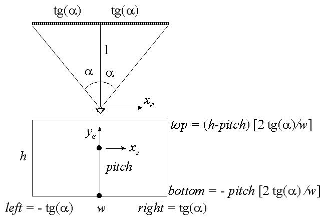
Note in Figure 6 that the factor h/w is required to maintain the aspect ratio between the window in the projection plane and the window where the image is to be drawn.
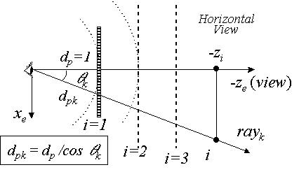
The depth computation in Algorithm 1 is expensive because it will vary differently for each screen column k. The primary reason for this is that for each column the distance dpk varies as shown in Figure 7. As dpk is an important value in Algorithm 1, each pixel column has its own sets of slopes and height variations. These coefficients differ from the central column only by the factor 1/cos(qk).
We can avoid computing slope and height variation for each column by correcting the distance measures in the rayk direction by the same factor 1/cos(qk). That is, if the distance i varies in slices as illustrated by the dashed lines (not the dotted circles) in Figure 7, we can use the slopes and the height variations with respect to i in column k using the same values we use for the central column. The way to implement this is to scale the unit vector (dx, dy) by the factor 1/cos(qk). Note that this produces the same gain in efficiency as the simplifications proposed by [LaMothe95] and [Freese+95] without the undesired distortions.
Even with the above simplification, depth computation for all slices i is still expensive, due to the non-linear nature of the conic projection. This relation can be obtained by the homogeneous matrix, P, given by equation (3). This matrix is used by OpenGL ( [Neider+93] and [Martha+94]) ) to transform between the eye and the screen coordinate systems.
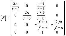 (3)
(3)where l, r, t, b, n, f stand for left, right, top, bottom, near and far, respectively.
Thus the screen coordinate, zs, can be computed from the eye coordinate, ze, by:
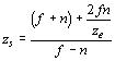 (4)
(4)OpenGL also provides a function called glDepthRange which specifies a linear mapping between the depth range [-1,1] and a chosen depth range. The default values for this new range are 0.0 for the near and 1.0 for the far distance. With these values, Equation (4) must be modified by:
With the above modifications, Algorithm 1 steps through the terrain model in slices parallel to the projection plane, as shown in Figure 7. The coordinate ze as a function of the slice i is then given by:
Replacing equations (6) in (4) and (4) in (5) we can have the depth value for each slice i given by
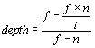 (7)
(7)It is important to note that this relation is invariant with the pixel column, the observer's position, and the view direction. That is, we can pre-compute all depths and store them in a vector of dimension far. It is important to note, however, that all these simplifications are only valid in the case where the view direction is horizontal, as shown in Figure 3.
We are assuming here that the depth vector has already been pre-computed
in the beginning of the program by the procedure shown in Algorithm 2.
DepthVector(n,f) {
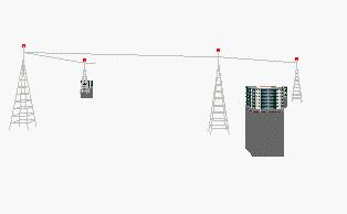
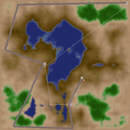
When the objects shown in Figure 9 are inserted in the terrain model according to the plan shown in Figure 10, the result are images of the type of the one shown in Figure 11.
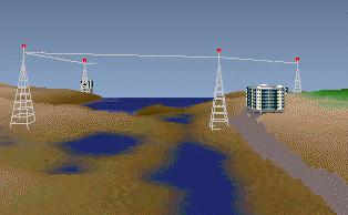
To evaluate the efficiency of the proposed strategy we measured the performance of the algorithm in two different computers: a PC Pentium 166 MHz, and a Silicon Indigo 2. The average time to generate a frame in two animated sequences is shown in Table 2. The first sequence renders the terrain with the objects ( Figure 11 ) and the second renders the terrain without the objects ( Figure 8 ). Average times were computed using 10 frames.
Note, in Table 2, that the time spent in depth computation in the Floating Horizon Algorithm is very small. The largest time is spent transferring the buffers to OpenGL. To load the color buffer we spent as much time as we did with the terrain rendering. To load the depth buffer we had to spend twice as much time as Floating Horizon did. The efficiency of the function responsible by these transfers, glDrawPixels, has been object of many discussions in the news group news:comp.graphics.api.opengl. It is conceivable that better results could be obtained with a more efficient version of this procedure.
Even with the low performance of the function glDrawPixels, the results obtained with the proposed strategy are far better than by making use of Z-Buffer to render the terrain. This fact reinforces the need for a specific algorithm to approach this class of problems.
| Terrain with objects | Terrain without objects | |||||||
| PC | SGI | PC | SGI | |||||
| Steps in the Algorithm | t(s) | t(%) | t(s) | t(%) | t(s) | t(%) | t(s) | t(%) |
| Floating Horizon | 0.05 | 23 | 0.18 | 51 | 0.04 | 50 | 0.13 | 76 |
| Z-Buffer load | 0.11 | 50 | 0.11 | 31 | - | - | - | - |
| Color Buffer load | 0.04 | 18 | 0.04 | 12 | 0.04 | 50 | 0.04 | 24 |
| Objects | 0.02 | 9 | 0.02 | 6 | - | - | - | - |
| Total Time | 0.22 | 100 | 0.35 | 100 | 0.08 | 100 | 0.17 | 100 |
| Frames/sec. | 4.6 | 3.0 | 14.1 | 5.9 | ||||
Although the aliasing problem was not severe in the examples presented here, the authors believe that it may became a serious concern if real aerial photos we used.
[Freese+95] P. Freese, More Tricks of the Game Programming Gurus, SAMS Publishing, 1995.
[Camara+96] G. Câmara et al., Anatomia de Sistemas de Informações Geográfica, 10a Escola de Computação, 1996.
[Frederick+96] P. Frederick et al., Visualização Interativa Tridimensional de Modelos de Terreno com Textura, Anais do IX SIBGRAPI, pp. 341-342, 1996.
[Martha+94] L. F. Martha et al., Uma Resumo das Transformações Geométricas para Visualização em 3D, Caderno de Comunicações do VII SIBGRAPI, pp. 9-12, 1994.
[Graf+94] K. Ch. Graf et al., Perspective Terrain Visualization - A Fusion of Remote Sensing, GIS, and Computer Graphics, Comput. & Graphics, Vol. 18, No. 6, pp. 795-802, 1994.
[tvcg+96] D. Cohen-Or et al., A Real-Time Photo-Realistic Visual Flytrough, ftp://ftp.math.tau.ac.il/pub/daniel/tiltan.ps.gz.
[Cohen+94] D. Cohen et al., Photorealistic Terrain Imaging and Flight Simulation, IEEE Computer Graphics and Applications, Vol. 14, No. 2, pp. 10-12, March, 1994.
[Paglieroni+94] D. Paglieroni et al., Height Distributional Distance Transform Methods for Height Field Ray Tracing, ACM Transactions on Graphics, Vol. 13, No. 4, pp. 376-399, October, 1994.
[Neider+93] J. Neider et al., OpenGL Programming Guide: the Official Guide Learnning OpenGL, release 1, Addison-Wesley Publishing Company, 1993.
[VistaPro] VistaPro, http://www.callamer.com/vrli/vp.html.
[Sawyer97] B. Sawyer, Skimming the Voxel Surface with NovaLogic's Commanche 3, Game Developer, pp. 62-70, April-May 1997.
[GuGaCa97] L. Guedes et al., Real Time Rendering of Photo-Texture Terrain Height Fields, Submitted to SiBGrapi'97.